MS Excel: Top 4 Freeze Panes In Excel

Added On: Jun 7, 2023

Last Update: Aug 17, 2023

Excel Freezing Panes is used to freeze or fix more than one column or row. Excel provides many ways for Excel users to scroll through Excel’s spreadsheet content.

There are many ways to freeze panes in Excel:

Freeze Top Row in Excel
Freeze First Column in Excel
Unfreeze Panes in Excel
Freeze a Specified Number of Rows and/or Columns

1. How To Freeze Top Row In Excel

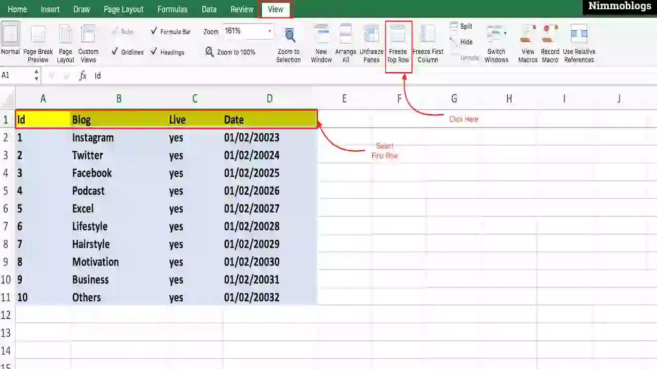
Excel provides a feature to just freeze the top row of the Excel worksheet. To do this simple procedure you just need to follow the steps mentioned below:

Select the first row of the worksheet.
Go to View option from the top ribbon.
Click on Freeze Top Row option.

2. How To Freeze First Column In Excel

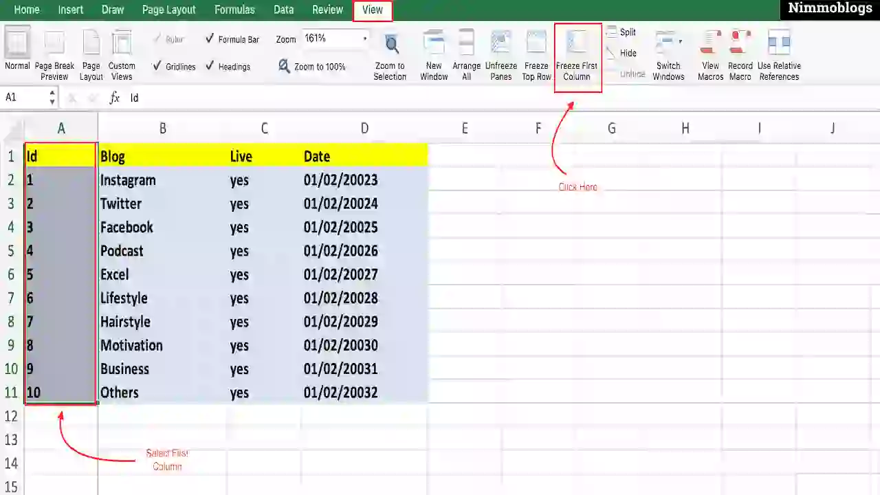
Excel provides a feature to just freeze the first column of the Excel worksheet. To do this simple procedure you just need to follow the steps mentioned below:

Select the first column of the worksheet.
Go to View option from the top ribbon.
Click on Freeze First Column option.

3. How To Freeze a Specified Number of Rows and/or Columns In Excel

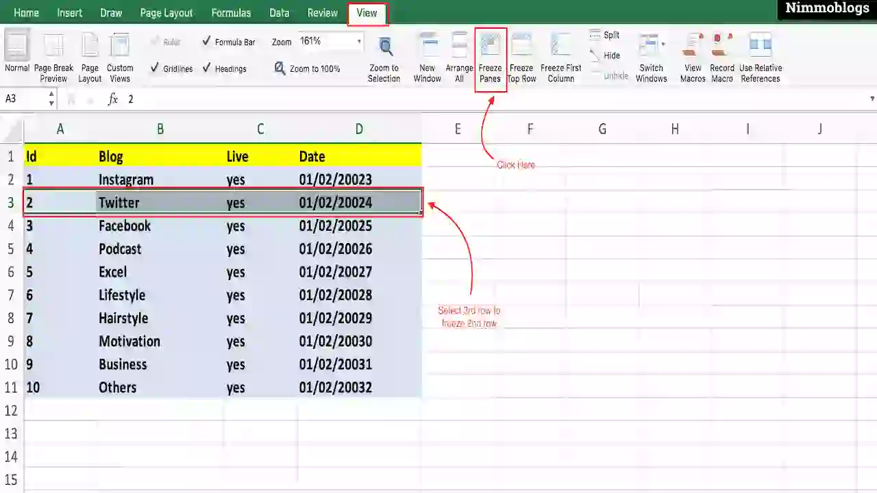
Excel also provides a way to freeze a particular column or row of the Excel worksheet. To do this simple procedure you just need to follow the steps mentioned below:

Select any row or column of the worksheet.
Go to View option from the top ribbon.
Click on Freeze Freeze Panes option.

4. How To Unfreeze Panes In Excel

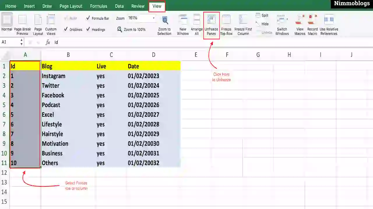
Excel provides a feature to unfreeze panes that you freeze for some reason in the Excel worksheet. To do this simple procedure you just need to follow the steps mentioned below:

Select the frozen column or row of the worksheet.
Go to View option from the top ribbon.
Click on Unfreeze Panes option.

Example For Each Method

Freeze the Top Row of a Spreadsheet

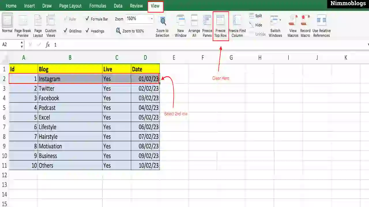
Excel Freeze Row means you select a top row and if you freeze all the Excel data you can scroll up and down but the frozen row will remain visible at the same point.

Here is an example to freeze the top row of the worksheet. This can be done by clicking on the Freeze Top Row option in the View section of the top ribbon. This option will freeze only the top row of the worksheet instead you have selected any other row.

Freeze the First Column of a Spreadsheet

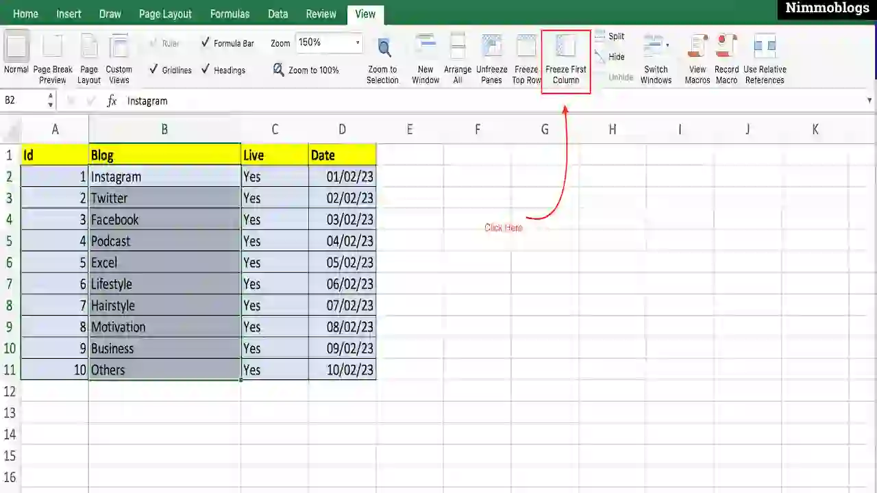
Excel Freeze Column option is used to freeze any column of the worksheet. Just select the column and go to the View tab and click on Freeze First Column.

When a column has been frozen then a black color line will be displayed on the worksheet on the right side of the column.

You can scroll Excel worksheet data towards left-to-right or right-to-left but the frozen column will remain in the same position. This option will freeze only the first column of the worksheet instead you have selected any other column. Here we freeze the First column of the worksheet but selected the 2nd column in the below image.

Freeze Top Row and First Column in Excel

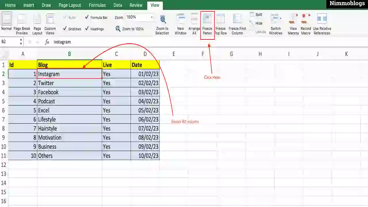
Excel Worksheet’s first column and top row can be frozen at the same time by only one option:

Select Cell B2.
Go to View tab in top ribben.
Click on Freeze Panes option.

Above steps to freeze the Top row and the first column will freeze both row and column at the same time.

It will look like that Excel worksheet displaying a black line below the top row and right of the first column. This black line will be displayed by Excel to highlight the frozen action on columns and rows.

Freeze Top 2 Rows in Excel

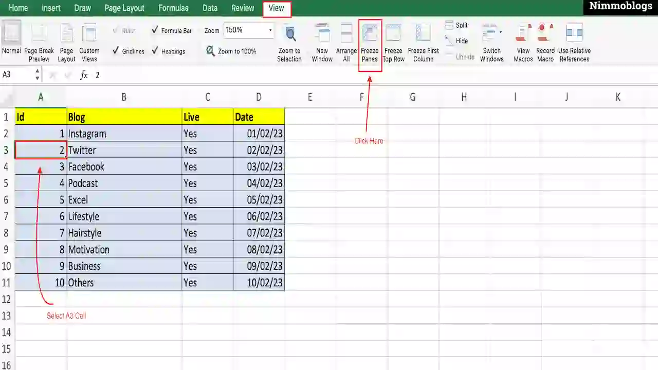
Excel Worksheet’s top two rows can be frozen at the same time by only one option:

Select Cell A3 of worksheet in Excel.
Go to View tab in top ribben.
Click on Freeze Panes option.

Above steps to freeze the Top two rows will freeze both rows at the same time.

There are no columns available towards the left of the A3 cell, so the frozen option will freeze the top 2 rows of the Excel worksheet.

It will look like that Excel worksheet displaying a black line below the top two rows. This black line will be displayed by Excel to highlight the frozen action on rows.