MS Excel: How To Use Conditional Formatting In Excel

Excel conditional formatting is basically used to change the cell’s formatting for below-mentioned criteria:

• Excel formatting based on the Value of the current cell.
• Excel formatting based on the Value of the other cell but the worksheet is the same.
• Excel formatting based on the result of the formula.

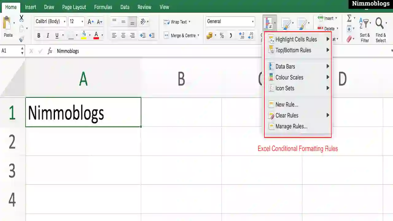
Excel Conditional Formatting Menu

Excel conditional formatting menu contains many rules, before going with these rules you need to select a cell in the Excel worksheet to apply this Conditional formatting.

• Select a cell in the Excel worksheet.
• Go to a Home ribbon at the top.
• Click on the Conditional Formatting option present in the middle.
• Or you can click on the drop-down on Conditional formatting to check the multiple rules of Conditional Formatting.
• You can choose one of the rules to apply on your cell or you can also create your own custom rule.

Excel Conditional Formatting Rules

• Highlight Cells Rules: This is used to apply specific conditions i.e. greater than, equal to, Duplicate Values, etc .
• Top/Bottom Rules: This is used to apply statistical conditions with respect to another cell of the current worksheet i.e. above average, within the top 10%, etc.
• Data Bars / Color Scales / Icon Sets: This is used to apply formatting with respect to other cells’ relation with the current cell.
• New Rule: This is used to apply the formatting of rules that are based on a result of the formula.

Using Multiple Conditions

Excel Conditional Formatting allows Excel users to define multiple conditions to apply multiple types of formatting to these. You have to specify a condition once, later you can define conditions by repeating the process to add a condition.

Excel also provides a way to manage or edit condition that was defined earlier, Just need to click on the Manage Rules option of the drop-down list of Excel Conditional Formatting menu. (Refer above image)

Excel Conditional Formatting rules in the drop-down list are listed in a manner, what does this order mean? This order means the first option in the list is tested first and then the next option will be tested and so on.

This order of Conditional formatting is needed when your Excel worksheet contains conditions that overlap e.g. B1>10, B1>5. This can be better understand by Common Error example, explained below.

Common Error

Excel’s conditional formatting is used once then it’s fine but if you use more than one condition for Excel Condition Formatting then you should know the conditions are tested in order as they are arranged in the Manage Rules window.

Example: if you wants to color a cell in red color if that contains a value greater than 10 and colored in orange if that cell contains a value greater than 5 but this definition will not work according to the expectations (This condition applies that test "Cell Value > 5" before the test "Cell Value > 10").

If you want the expected result for this condition, then apply "Cell Value > 10" first and place the condition "Cell Value > 5" second.