Excel  Excel
Excel
MS Excel: How To Create Excel Drop Down List
Added On:
Last Update:
Excel Drop Down list is a very satisfying way to select required data from multiple data. Using Excel Drop Down list Excel users can save time instead of entering data manually in the worksheet of Excel.
Drop-Down lists are used mostly to get information from users by form. Whether you running a home or a business, everybody wants things to be organized. So, this Excel Drop Down list is a way to organize data and save time.
To use Excel drop-down list, do the following steps to create a drop-down in the worksheet:
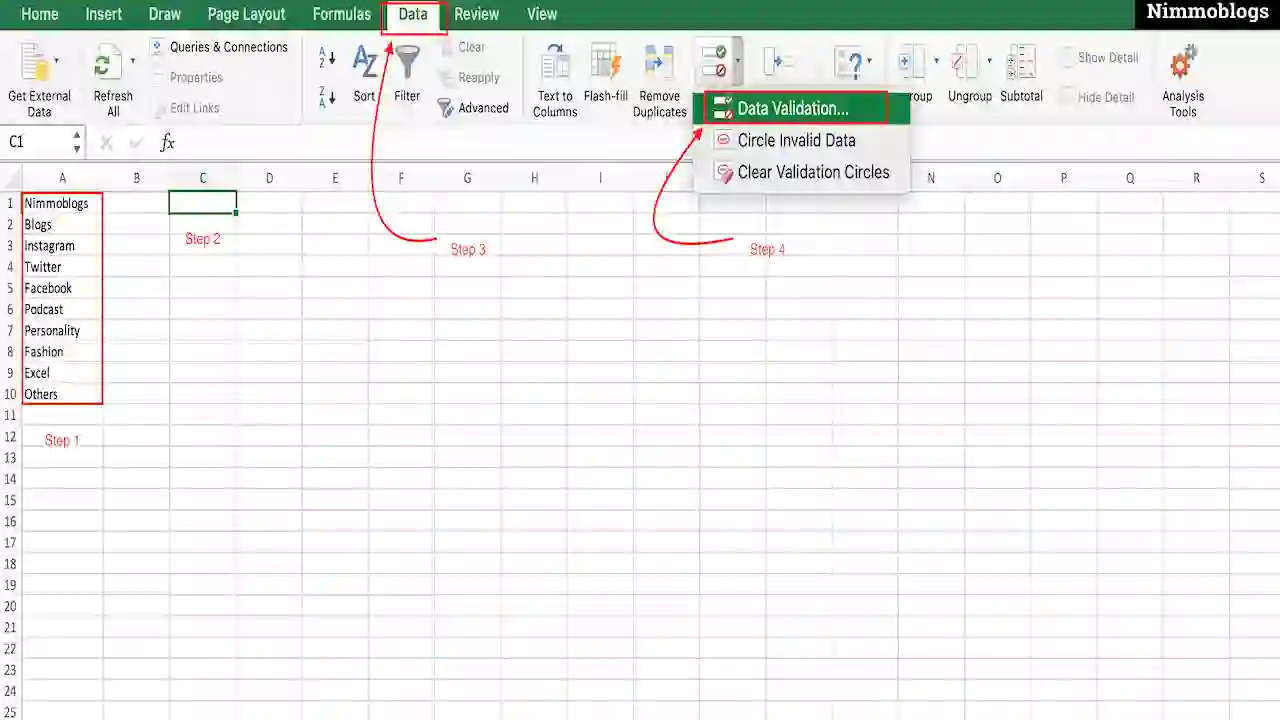
- First, you have to some values of data (values you wants to show in the drop-down list) into columns of the worksheet in Excel as in the image data entered in A1-A10
- Select any one cell A1-A10, that you want to make visible in the Drop-Down list.
- Go to the "Data" tab at the middle top and click on "Data Validation" Then you will have 3 options, now click on the first option named "Data Validation".
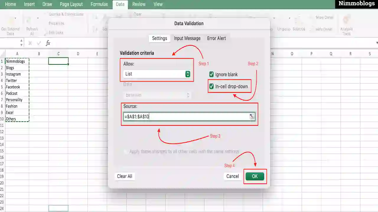
- A dialogue will open when you clicked on the "Data Validation" option. There are many options available, go through the below steps for more clarification:
- In the "Allow" Field of the pop-up box, many options are available but you have to choose "List" from the multiple options.
- There is an "In-cell drop-down" option available at the right of the "Allow" field, make sure that option should be checked.
- Now, come down to the source field, where you have to give the cell number where you type the values (i.e. A1-A10 cells).
- Click on the "Ok" button when you are done with inputting cell reference.
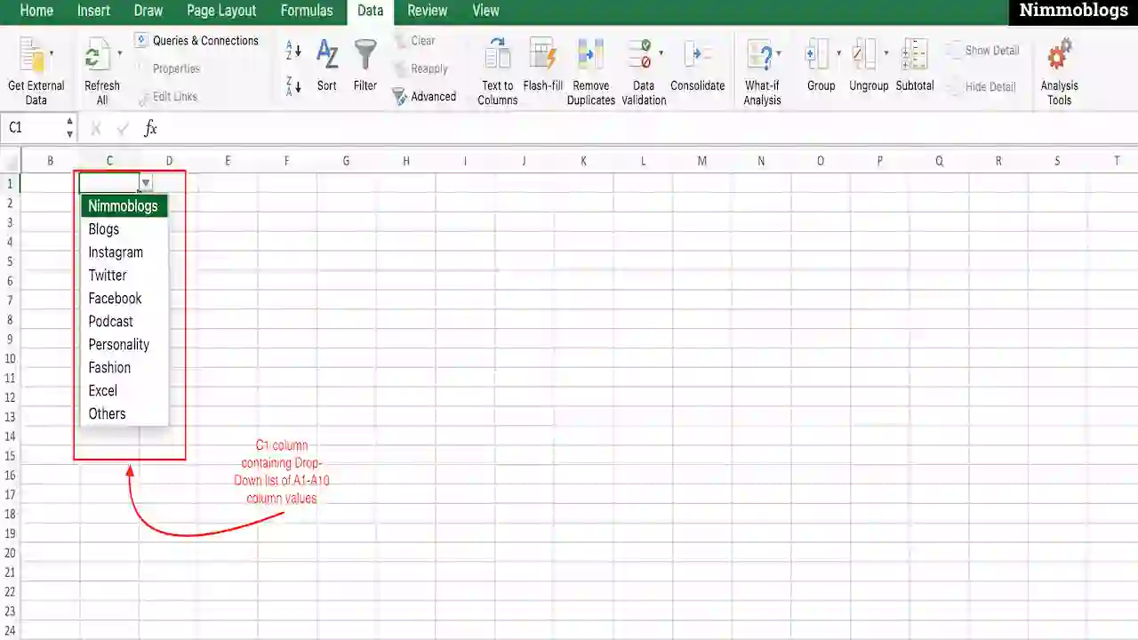
- Now, your drop-down list is created in the column where you select the empty field (i.e. C1). The C1 column now has a drop-down symbol that contains the list you created in the A1-A10 cells of the worksheet.
- If you want you can hide Column A and now also C1 column has a drop-down list.
|
|

Goal Setting: How To Set Goal In Life

Podcast: How To Cancel Spotify Premium

Podcast: Podcast That Should Listen

Podcast: What Is Google Podcast

Podcast: What Is Podcast And How Does It Works

Time Management: Good Time Management Skills

Time Management: How To Improve Time Management Skills

Top 25 Ways To Increase Productivity

Robotics: What Is Robotics And How Does It Work

Positive Thoughts: Positive Thoughts Can Change Your Life

How To Become Rich With No Money

Top 5 Ways To Become A Rich

Communication: Top 7 Ways To Communicate Effectively

Personality Development Tips For Men

Personality Development Tips For Woman
About Us,
T&C,
Privacy,
Contact Us,
Sitemap
©2025 Nimmoblogs
All Right Reserved.
Made with by Hina Aggarwal
©2025 Nimmoblogs
All Right Reserved.
Made with
by Hina Aggarwal